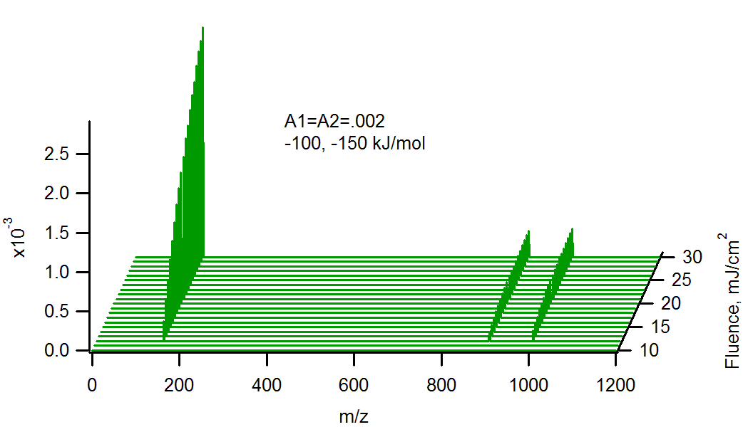
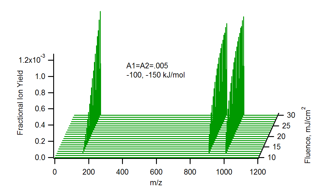
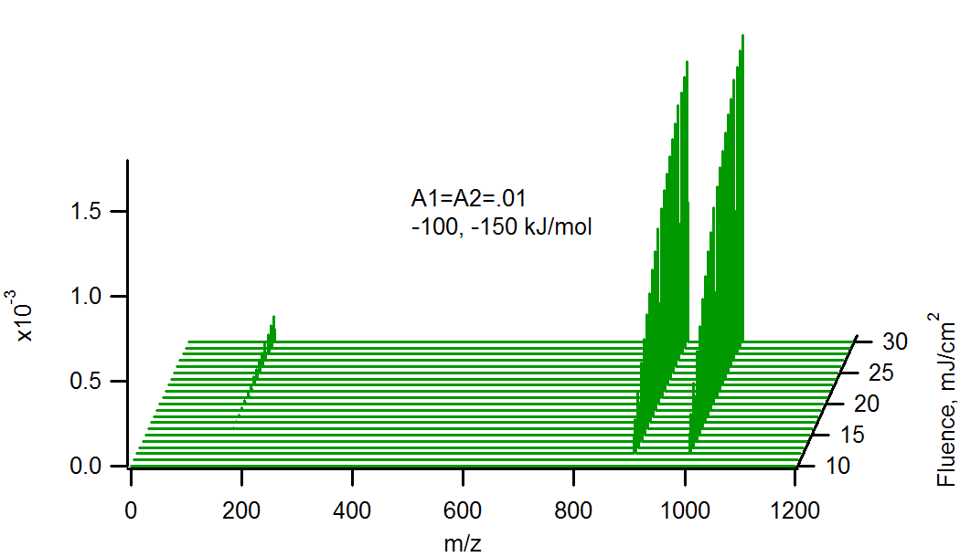
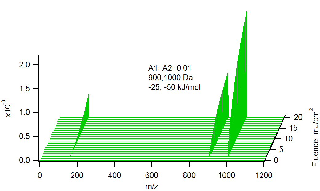
The example spectra below include the effect of laser fluence (right axis) as well as at least one other effect.

Analyte Concentration
The relative signal strengths of matrix and analytes depend on the total amount of analyte present:

Calculated MALDI spectra of matrix (m/z 154, DHB), and two analytes (m/z 900 and 1000), vs. laser fluence at 355 nm, 5 ns pulse width. The analytes are present in equal mole fractions, but differing charge transfer energetics with the matrix primary ions. The heavier analyte reacts more energetically than the lighter (150 vs 100 kJ/mol). Note the matrix suppression effect at the highest analyte concentration and lowest fluence.

The corresponding analyte/analyte and matrix/analyte ratios are shown next.

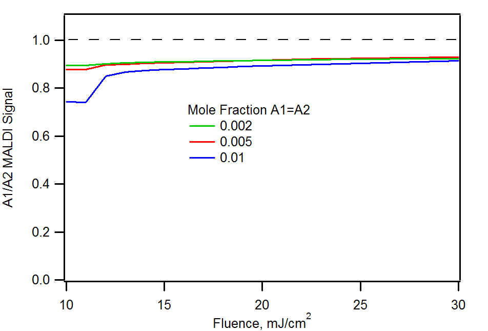
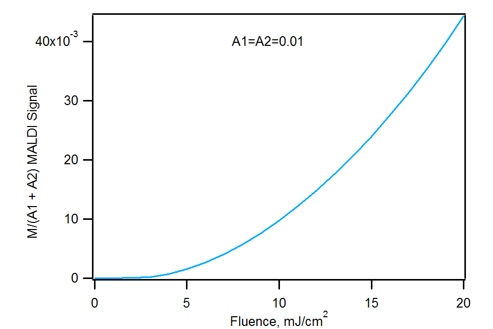
Analyte/analyte and matrix/analyte signal ratios corresponding to the previous figure. Note that the A1/A2 ratio is always skewed in favor of the most reactive analyte. The matrix/analyte figure is for an A1=A2=0.01 mole fraction.

Because analyte 2 (m/z 1000) has more favorable reaction thermodynamics with the matrix, it is always favored. The A1/A2 ratio never reaches the correct value of 1, although it improves at higher laser fluence. This is because a greater supply of primary matrix ions reduces the importance of competition between the analytes for charge. The right panel shows how sufficient analyte can react quantitatively with the available primary matrix ions, leaving no matrix signal at all. As more primary ions become available, due to increase laser energy deposition, there is insufficient analyte to fully suppress the matrix.

Analyte Molecular Weight
Because heavier analytes have a physically larger collision cross section (an effect which plays a large role in ion mobility spectrometry), they also react more efficiently with primary matrix ions. They are also initially in contact with more matrix before the sample is ablated, so there is a bigger chance of being near an ionized matrix from the start. Both these effects lead to a distinct enhancement of relative ion signal for larger ions. Unfortunately the typical secondary electron multiplier detectors of most ToF instruments loose sensitivity for large ions at an even faster rate!

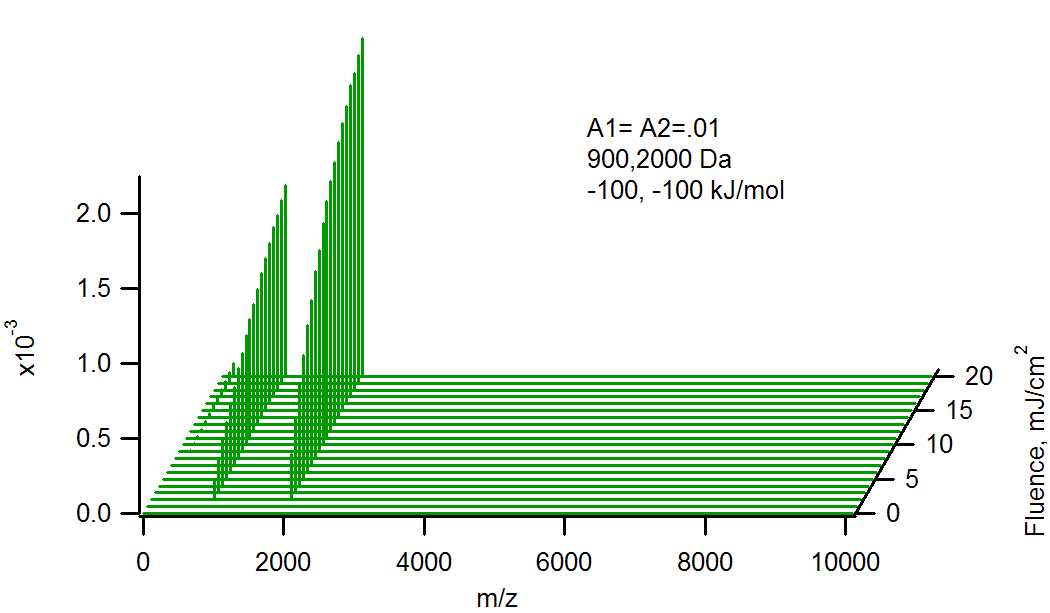
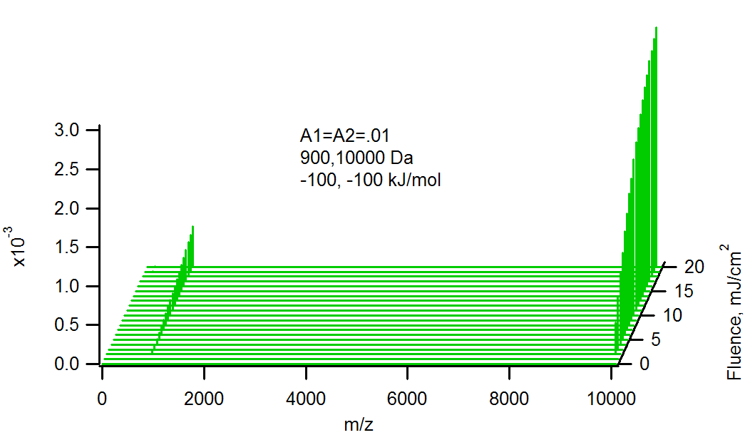
Effect of molecular weight on relative analyte ion signals. Heavier molecules are larger, and have a larger probability of reacting with primary matrix ions.

Charge Transfer Thermodynamics
The next graphs show how the absolute and relative matrix and analyte signals depend on the driving force for charge transfer from primary matrix ions to analyte acceptors. This is for reactions with kinetics similar to that of proton transfer. Transfer of electrons may well be faster (at least up to the Marcus inversion point), and that of heavier ions slower.

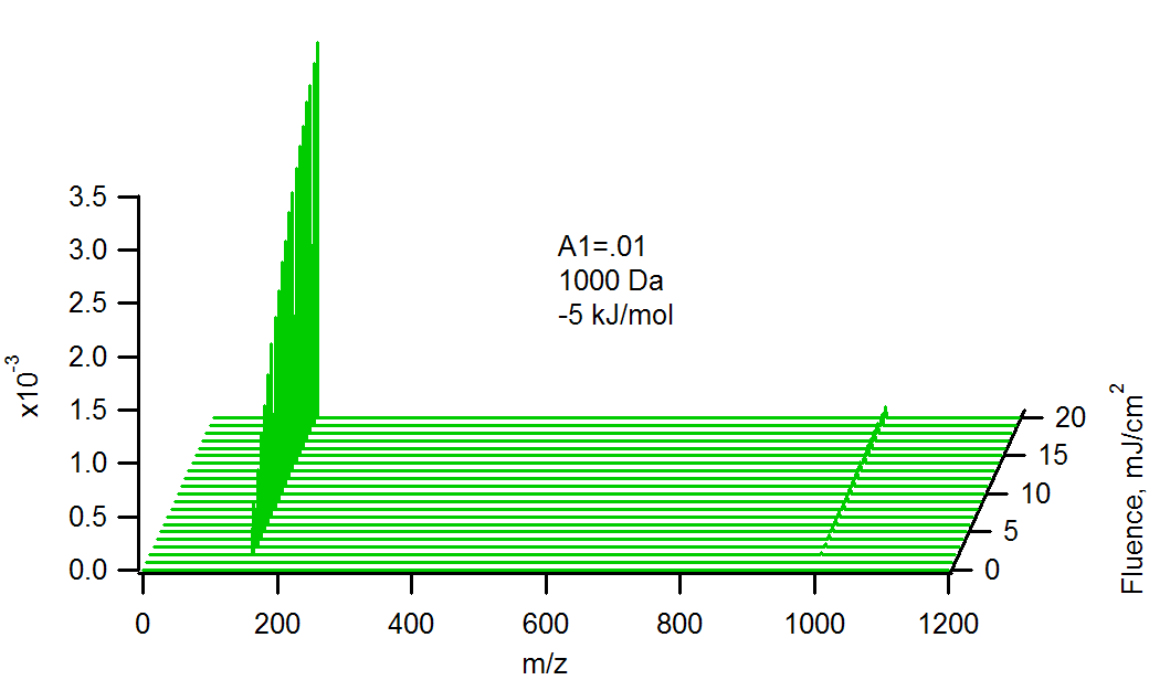
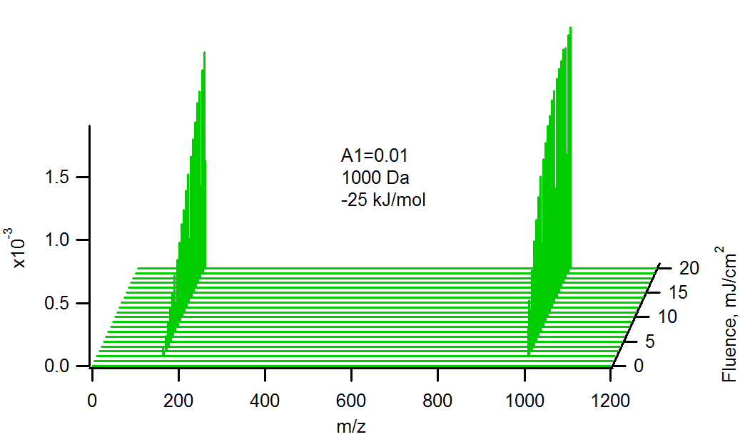
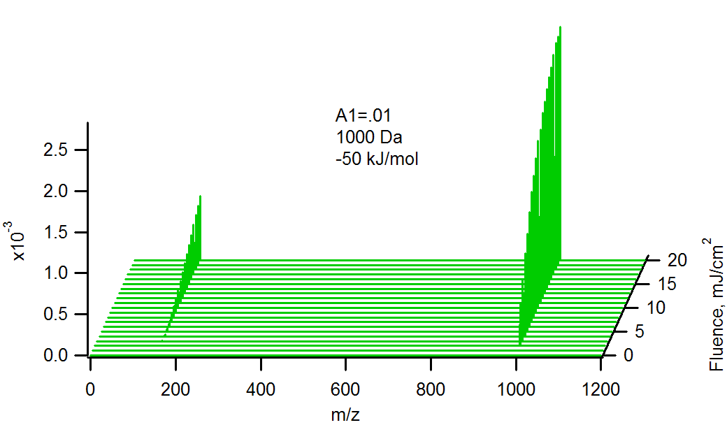
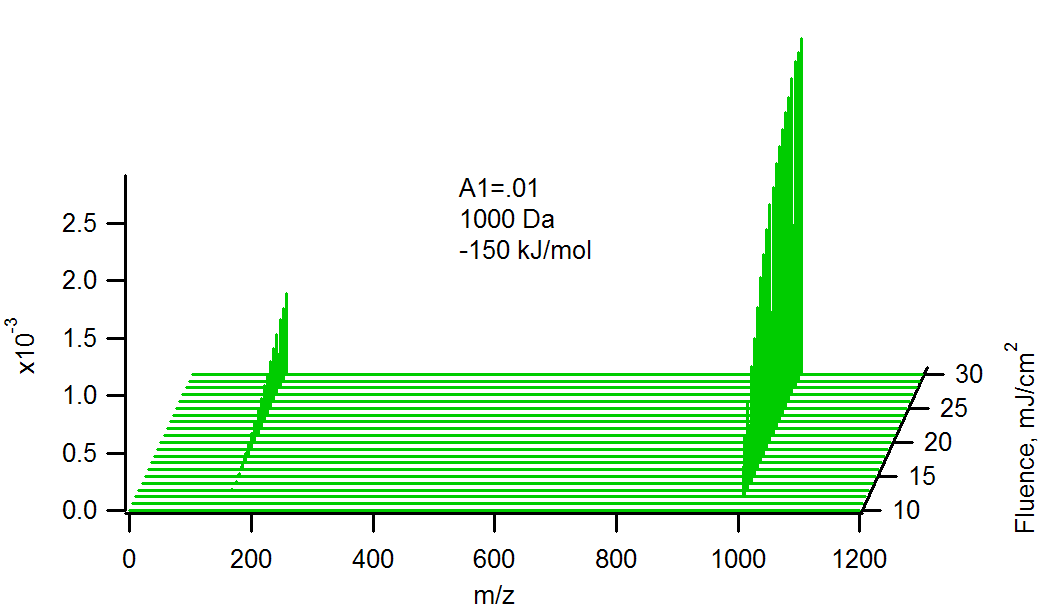
Effect of charge transfer reaction ΔG on matrix and analyte ion signals (one analyte). Reaction with matrix is efficient except at low ΔG.

The effect of reaction free energy on two analytes is shown next:

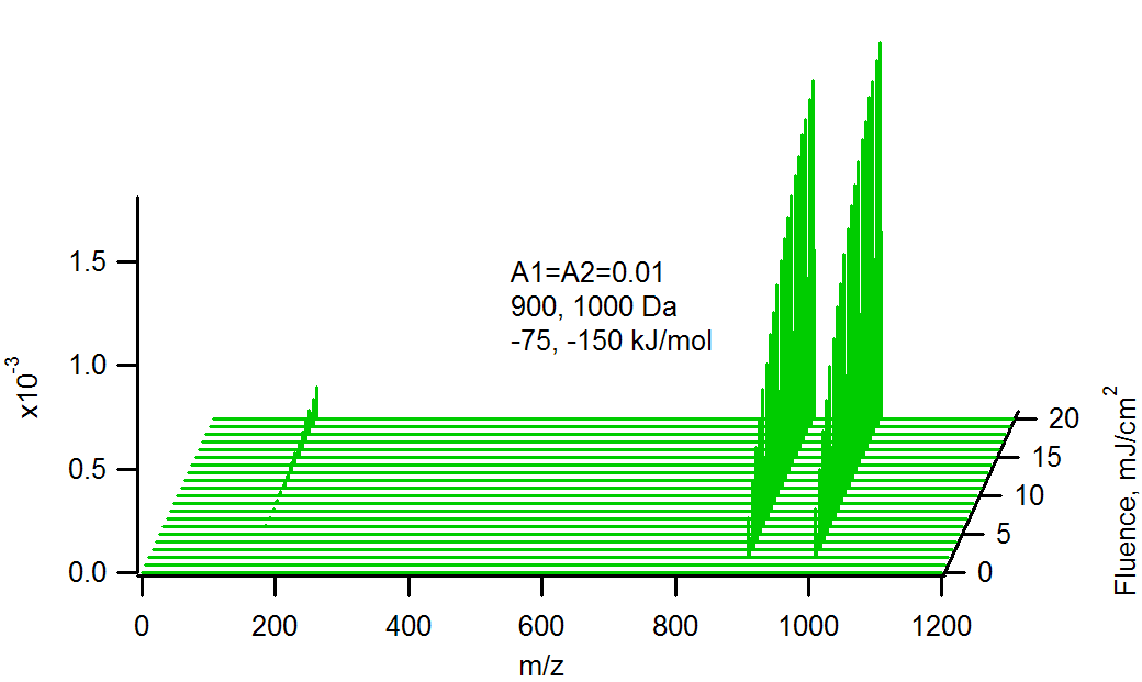
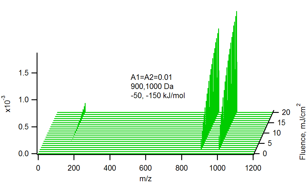
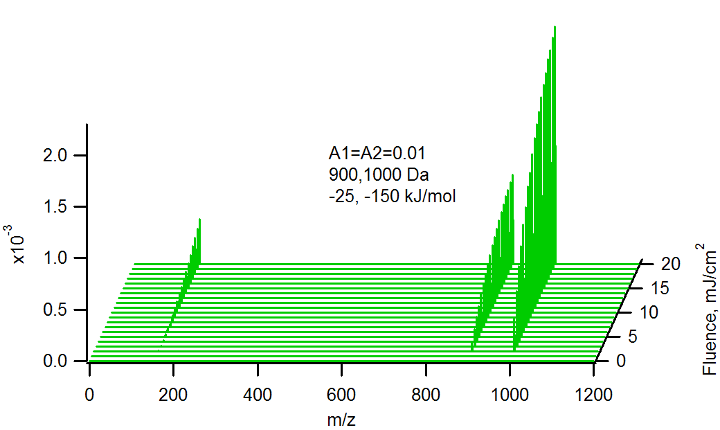
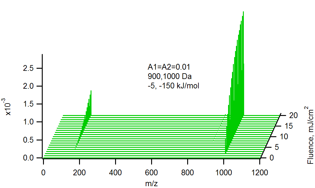
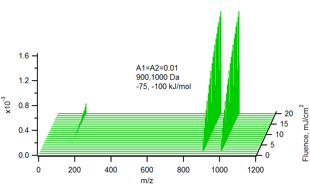
Effect of charge transfer reaction ΔG on matrix and analyte ion signals (two analytes). Reaction with matrix is efficient except at low ΔG.

Positive / Negative Analyte Ratios

See these papers for the full story:
Int. J. Mass Spectrom., vol. 273, pp. 84-86 (2008)
Final submitted manuscript

and:
Int. J. Mass Spectrom., vol. 285, pp. 105-113 (2009)
Final submitted manuscript

The relative strengths of analyte MALDI signals in positive vs. negative polarities is not only useful to plan an experiment, but is also a window on ion formation processes. If either the matrix or the analyte is changed, the secondary reaction thermodynamics also change, in both polarities. Comparing measured analyte signals from a set of matrixes and analytes should show a consistent, systematic trend. By taking the ratio of positive and negative ions we test the consistency of our models for two sets of reactions simultaneously.

It is not easy to get accurate, comparable data of this kind. Very few instruments can measure positive and negative ions from the same ablation event, so it is necessary to measure the polarities separately, then carefully correct for numerous factors. The published data of this type is shown below, but it should be noted that much better data has been obtained recently by the Owens group and will hopefully be published soon.

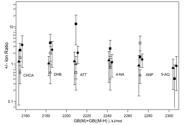
Positive/negative analyte ion ratios for some analytes and six matrixes. The horizontal axis is the difference between the matrix gas phase basicity (ΔG of proton attachment to the neutral) and the basicity of its conjugate base (ΔG of separation into a proton and anion). Adapted from Int.J. Mass Spectrom. vol. 268 p. 122 (2007).

The data do show a consistent trend: a flat one a value very close to unity. If the plume were in something like equilibrium (remember true equilbrium would mean no ions at all), this would not be expected, since the horizontal axis spans 200 kJ/mol. The relation ΔG=-RTln(K) tells us that the equilibrium constant, K, should shift quite a lot over this range of ΔG.

It turns out that the two step model can easily explain and reproduce this result. It is found to be an excellent example of the fact that kinetics in the MALDI plume also matter, it isnt just a question of thermodynamics.

As discussed in this chapter, an Arrhenius equation is used to describe the charge transfer kinetics, which includes a frequency factor and an activation energy. The activation energy is derived from the reaction free energy by a nonlinear free energy relationship. This is a fixed quantity. The frequency factor is related to the rate of collisions between the reaction partners. It therefore depends on the plume temperature and density. Since these change during the event, the reaction rates are modulated. The next figure shows some examples.

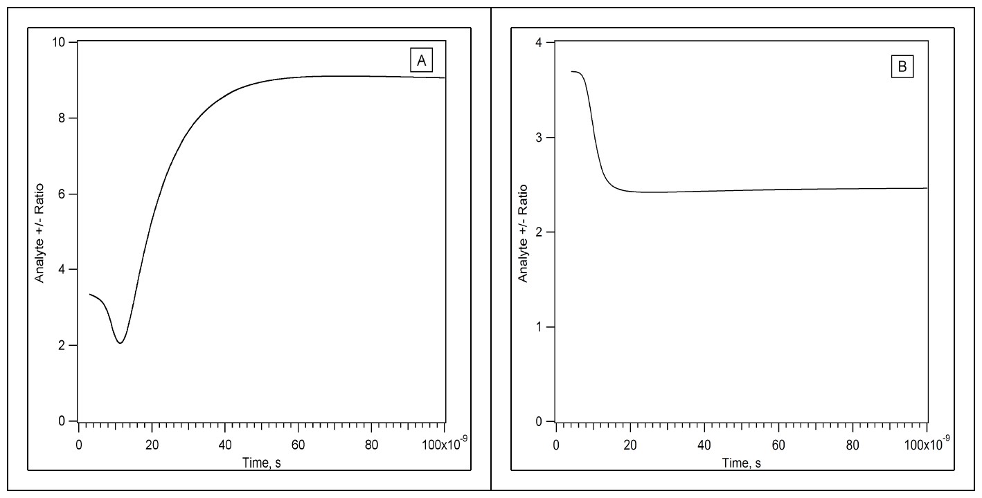
Time evolution of the positive/negative analyte ion ratio in the two step model. Matrix–analyte forward reactions initially proceed quickly in the dense sample, leading to an early imbalance. Slow reverse reactions during the later plume expansion hinder return toward equilibrium. In panel (A) the initial analyte mole fraction is 0.01, in panel (B) it is 0.0001.

As is apparent, the ratio can change quite a lot during the MALDI event, until it finally becomes "frozen" because the plume has become too dilute. As the above examples show, the early dense period is when the biggest changes occur. If the forward secondary reaction (donation of charge to the analyte, from the primary ions) is favorable, it goes far toward completion in the early period. This is true in both polarities, so the positive and negative analyte ion concentrations are about the same, the ratio near 1. If the forward reactions are fast, the reverse reactions are usually slow (unfavorable ΔG), so the system relaxes slowly toward equilibrium. But the plume expands too fast for the two polarities to get close to equilibrium (note that the ions in one polarity may be much closer to equilibrium than are ions of different polarity).

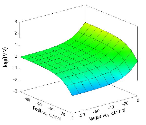
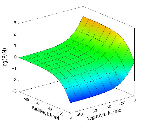
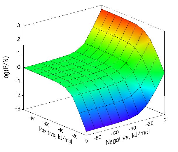
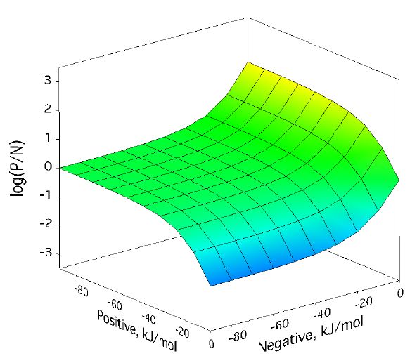
Positive/negative analyte ion ratio as a function of matrix–analyte reaction free energies, and at three analyte mole fractions: 0.0001 in (left), 0.001 in (center), and 0.01 in (right). The laser fluence was 17 mJ/cm2. Approach to PNAIR equilibrium is faster at higher analyte mole fractions, but the plateau is present in every case.

For a broad region where both positive and negative secondary reactions are more favorable than about -30 kJ/mol, the p/n ratio expected from the model is quite near one. This doesnt depend much on analyte concentration. As the next figure shows, it also doesnt depend much on laser fluence, the other main MALDI experimental variable.

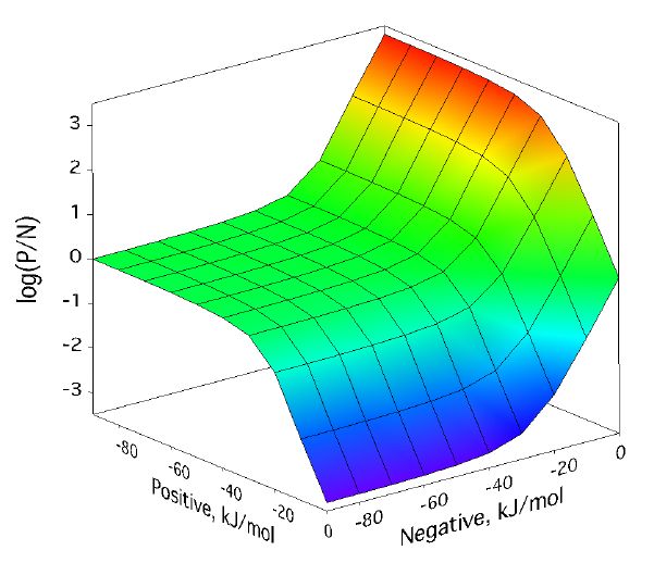
Positive/negative analyte ion ratio as a function of matrix–analyte reaction free energies, at three laser fluences: 12 mJ/cm² (left), 17 mJ/cm² (center), and 22 mJ/cm² (right). The analyte mole fraction was 0.001.

So the data of the first figure of this section is easy to understand- the forward reactions in both polarities are at least moderately favorable, the two step model predicts a ratio close to 1, regardless of significant experimental inconsistencies in concentration or laser fluence.

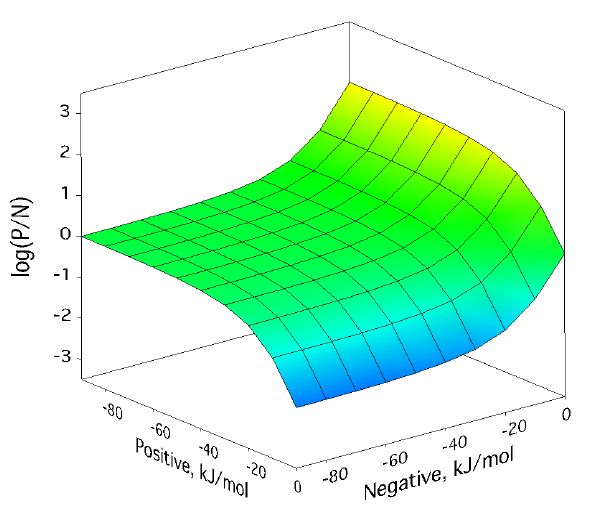
Of course, not only are single analytes subject to kinetic limitations on their secondary reactions, there will be similar effects when comparing two or more analytes. Several effects are included in the following graph:

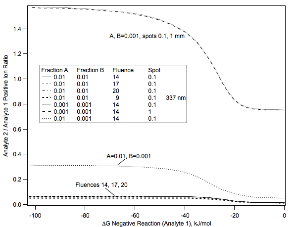
Positive/negative analyte ion ratio Ion ratio of two analytes, in positive mode, as a function of negative ion secondary reaction ΔG for analyte 1, and several other parameters. Efficient negative ion reaction depletes neutral analyte, reducing the ion ratio in positive polarity. Analyte suppression is therefore most effective when secondary reactions in the opposite polarity are unfavorable. The positive secondary reaction ΔG for analyte 1 was −100 kJ/mol. The positive secondary reaction ΔG for analyte 2 was −30 kJ/mol, and the negative reaction ΔG −10 kJ/mol. The laser wavelength was 355 nm, except as indicated. The spot diameters are in mm, and the fluences in mJ/cm² .

More Examples?
If you have a question which is not answered by these examples, contact the author.